Understanding Single-Layer Neural Networks
Key Concepts
-
Neuron (Perceptron)
A neutron is the fundamental unit of the network. Each neuron computes a weighted sum of inputs plus a bias, then applies an activation function (e.g. step, sigmoid) -
Input Layer
The input layer accepts the raw data features. Each input is multiplied by an associated weight and passed to the neuron. It is often represented by a vector $\mathbf{x} \in \mathbb{R}^n$. - Weights and Bias
- Weights represent the importance of each input feature. It is often represented by a vector $\mathbf{w} \in \mathbb{R}^n$.
- Bias allows shifting the decision boundary away from the origin.
-
Linear Combination
\[z = \mathbf{w}^\top \mathbf{x} + b\]
The neuron computes:Where $\mathbf{w}$ = weight, $\mathbf{x}$ = input, $b$ = bias
-
Activation Function
The activation function introduces non-linearity (in classic perceptron often a step function). It determines the output class or value. Without it, the network is just a linear model. -
Output Layer
It provides the final prediction. In a single-layer network, there is only one set of weights between the input and output (no hidden layer). -
Decision Boundary
The hyperplane separating classes in the input space. In a single-layer network, this boundary is always linear. -
Ground Truth
The true label of the data point, denoted as $y_{\text{true}} \in {0,1}$. It represents the actual class assigned in the dataset. -
Prediction
The model produces $\hat{y}$, derived from the probability $p$. Typically, $\hat{y} = 1$ if $p \geq \tau$, else $\hat{y} = 0$. -
Loss Function (Cross-Entropy)
\[\mathcal{L}(y_{\text{true}}, p) = - \big[ y_{\text{true}} \cdot \log(p) + (1 - y_{\text{true}}) \cdot \log(1 - p) \big]\]
To train the model, the predicted probability $p$ is compared with the ground truth $y_{\text{true}}$ using the binary cross-entropy loss:This loss penalises large differences between the predicted probability and the actual label. Minimising $\mathcal{L}$ adjusts the weights $w$ and bias $b$ to improve classification performance.
-
Backpropagation
Gradients of the loss are propagated back to update the weights and bias. -
Gradient Descent
\[\mathbf{w} := \mathbf{w} - \eta \frac{\partial \mathcal{L}}{\partial \mathbf{w}}, \quad b := b - \eta \frac{\partial \mathcal{L}}{\partial b}\]
The parameters are updated iteratively to minimise the loss:where $\eta > 0$ is the learning rate controlling the step size.
Architecture of a Single-Layer Neural Network
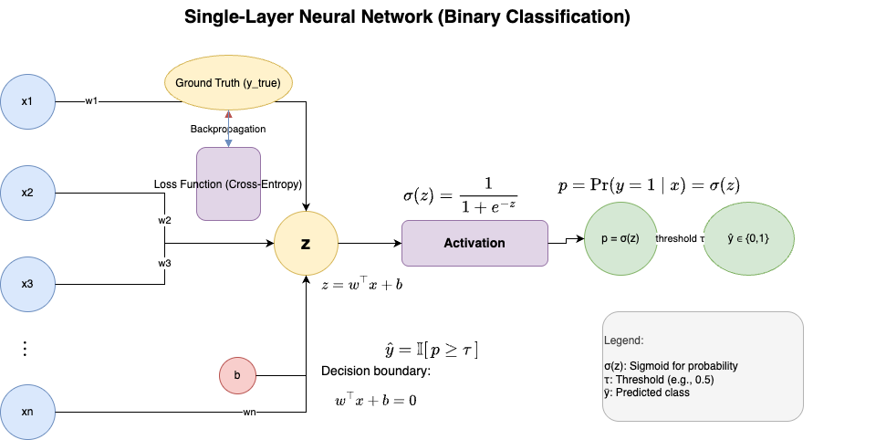
This diagram illustrates a single-layer neural network for binary classification. The input is represented as a feature vector $\mathbf{x} \in \mathbb{R}^n$, and the parameters of the model are a weight vector $\mathbf{w} \in \mathbb{R}^n$ and a bias term $b \in \mathbb{R}$. The linear combination is computed as $z = \mathbf{w}^\top \mathbf{x} + b$. This value is then passed through a sigmoid activation function $\sigma(z) = \frac{1}{1+e^{-z}}$, which outputs a probability $p = \Pr(y=1 \mid \mathbf{x}) = \sigma(z)$, representing the likelihood that the class label $y$ equals 1. Finally, the probability is compared to a threshold $\tau$ (e.g., 0.5) to produce the predicted class label $y \in {0,1}$. The decision boundary of this model is defined by $\mathbf{w}^\top \mathbf{x} + b = 0$.