Multi-Layer Perceptron Neural Networks
Key Concepts
- Hidden Layers
An MLP contains one or more hidden layers between the input and output.
Each hidden layer applies a linear transformation followed by a non-linear activation function:
\(H_\ell = f_\ell(H_{\ell-1} W_\ell + \mathbf{1} b_\ell^\top)\)
where:- $H_{\ell-1}$ is the previous layer’s output (with $H_0 = X$).
- $W_\ell, b_\ell$ are the weight matrix and bias vector for layer $\ell$.
- $f_\ell(\cdot)$ is a non-linear activation (e.g., ReLU, tanh, sigmoid).
- Deep Representations
Multiple hidden layers allow the network to learn hierarchical feature representations.- Early layers capture low-level patterns (e.g., edges in images).
- Deeper layers capture higher-level abstractions (e.g., object shapes).
- Activation Functions
Unlike the single-layer perceptron (which often uses only sigmoid), MLPs commonly use:- ReLU: $f(x) = \max(0, x)$ (default in modern deep learning).
- Tanh: rescales input to $[-1,1]$.
- Sigmoid: mainly used in the output layer for binary classification.
- Output Layer
- For binary classification: sigmoid function produces $p = \sigma(z)$.
- For multi-class classification: softmax produces probability distribution over $K$ classes:
\(p_k = \frac{\exp(z_k)}{\sum_{j=1}^K \exp(z_j)} \quad (k=1,\dots,K)\)
- Loss Function (Extension)
- Binary case: same as SLP (binary cross-entropy).
- Multi-class case: categorical cross-entropy with one-hot labels:
\(\mathcal{L} = -\frac{1}{m} \sum_{i=1}^m \sum_{k=1}^K y_{i,k} \log p_{i,k}\)
-
Backpropagation Through Layers
The error signal is propagated backward through each layer using the chain rule, enabling gradient computation for all parameters:
\(\frac{\partial \mathcal{L}}{\partial W_\ell}, \quad \frac{\partial \mathcal{L}}{\partial b_\ell}, \quad \ell = 1,\dots,L\) - Universal Approximation
With enough hidden units, an MLP can approximate any continuous function on a compact domain.
This property underlies its power as a general-purpose function approximator.
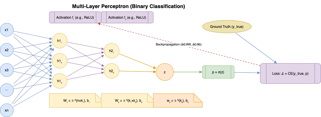
Architecture of a Multi-Layer Perceptron Neural Network
Formulas
- Input
- Mini-batch input: \(X \in \mathbb{R}^{m \times n}\)
- where:
- $m$ = batch size
- $n$ = number of features
- Parameters: \(W_1 \in \mathbb{R}^{n \times k_1}, \quad b_1 \in \mathbb{R}^{k_1}\) \(W_2 \in \mathbb{R}^{k_1 \times k_2}, \quad b_2 \in \mathbb{R}^{k_2}\) \(w_3 \in \mathbb{R}^{k_2}, \quad b_3 \in \mathbb{R}\)
-
Forward Propagation
-
Hidden Layer 1 \(H_1 = f_1\!\big( X W_1 + \mathbf{1} b_1^\top \big) \quad \in \mathbb{R}^{m \times k_1}\)
-
Hidden Layer 2 \(H_2 = f_2\!\big( H_1 W_2 + \mathbf{1} b_2^\top \big) \quad \in \mathbb{R}^{m \times k_2}\)
-
Output Pre-activation \(z = H_2 w_3 + b_3 \mathbf{1} \quad \in \mathbb{R}^{m}\)
-
Sigmoid Activation \(p = \sigma(z) = \frac{1}{1 + e^{-z}} \quad \in \mathbb{R}^{m}\)
-
-
Prediction \(\hat{y}_i = \begin{cases} 1, & \text{if } p_i \geq \tau \\ 0, & \text{if } p_i < \tau \end{cases}\) with threshold $\tau = 0.5$.
-
Loss Function (Binary Cross-Entropy)
For a batch: \(\mathcal{L} = -\frac{1}{m} \sum_{i=1}^m \Big( y_i \log(p_i) + (1-y_i)\log(1-p_i) \Big)\)
Vectorised form: \(\mathcal{L} = -\frac{1}{m} \Big[ y^\top \log p + (1-y)^\top \log (1-p) \Big]\)
-
Backpropagation (Gradients)
-
Output layer: \(\frac{\partial \mathcal{L}}{\partial z} = p - y \quad \in \mathbb{R}^m\)
-
Gradients for output weights and bias: \(\frac{\partial \mathcal{L}}{\partial w_3} = \frac{1}{m} H_2^\top (p-y)\) \(\frac{\partial \mathcal{L}}{\partial b_3} = \frac{1}{m} \mathbf{1}^\top (p-y)\)
-
Hidden layers (chain rule with chosen activations $f_1, f_2$).
-
-
Parameter Update (Gradient Descent)
With learning rate $\eta > 0$: \(W_\ell \leftarrow W_\ell - \eta \frac{\partial \mathcal{L}}{\partial W_\ell}, \quad b_\ell \leftarrow b_\ell - \eta \frac{\partial \mathcal{L}}{\partial b_\ell} \quad (\ell = 1,2,3)\)
Implementation and Explanation
This section contrasts a from-scratch NumPy implementation with an equivalent PyTorch model. Both pipelines share the same data preprocessing, hyperparameters, and evaluation workflow so their learning curves can be compared directly.
Custom Version
The custom network is assembled from lightweight building blocks: Linear, ReLU, and CrossEntropy. Each layer stores the activations it needs for the backward pass, computes gradients manually, and updates its parameters via SGD in the step routine. Utility helpers handle one-hot encoding, mini-batch iteration, normalisation, and accuracy tracking so the training loop mirrors a framework-driven workflow while keeping every tensor transformation explicit.
1
2
3
4
5
6
7
8
9
10
11
12
13
14
15
16
17
18
19
20
21
22
23
24
25
26
27
28
29
30
31
32
33
34
35
36
37
38
39
40
41
42
43
44
45
46
47
48
49
50
51
52
53
54
55
56
57
58
59
60
61
62
63
64
65
66
67
68
69
70
71
72
73
74
75
76
77
78
79
80
81
82
83
84
85
86
87
88
89
90
91
92
93
94
95
96
97
98
99
100
101
102
103
104
105
106
107
108
109
110
111
112
113
114
115
116
117
118
119
120
121
122
123
124
125
126
127
128
129
130
131
132
133
134
135
136
137
138
139
140
141
142
143
144
145
146
147
148
149
150
151
152
153
154
155
156
157
158
159
160
161
162
163
164
import numpy as np

np.random.seed(8)


class Linear:
    def __init__(self, in_features, out_features):
        self.W = np.random.randn(out_features, in_features) * np.sqrt(2.0 / in_features)
        self.b = np.zeros((out_features, 1))

    def forward(self, x):
        self.x = x
        return self.W @ x + self.b

    def backward(self, grad_output):
        batch_size = grad_output.shape[1]
        self.dW = grad_output @ self.x.T / batch_size
        self.db = np.sum(grad_output, axis=1, keepdims=True) / batch_size
        return self.W.T @ grad_output


class ReLU:
    def forward(self, x):
        self.mask = x > 0
        return np.maximum(0, x)

    def backward(self, grad_output):
        return grad_output * self.mask


class CrossEntropy:
    def forward(self, logits, labels):
        shifted = logits - np.max(logits, axis=0, keepdims=True)
        exp_scores = np.exp(shifted)
        probs = exp_scores / np.sum(exp_scores, axis=0, keepdims=True)
        self.probs = probs
        self.labels = labels
        return -np.sum(labels * np.log(probs + 1e-15)) / labels.shape[1]

    def backward(self):
        return (self.probs - self.labels) / self.labels.shape[1]


class ThreeLayerNN:
    def __init__(self, input_dim, hidden_dim1, hidden_dim2, output_dim):
        self.fc1 = Linear(input_dim, hidden_dim1)
        self.act1 = ReLU()
        self.fc2 = Linear(hidden_dim1, hidden_dim2)
        self.act2 = ReLU()
        self.fc3 = Linear(hidden_dim2, output_dim)

    def forward(self, x):
        z1 = self.fc1.forward(x)
        a1 = self.act1.forward(z1)
        z2 = self.fc2.forward(a1)
        a2 = self.act2.forward(z2)
        logits = self.fc3.forward(a2)
        return logits

    def backward(self, grad_output):
        grad_hidden2 = self.fc3.backward(grad_output)
        grad_hidden2 = self.act2.backward(grad_hidden2)
        grad_hidden1 = self.fc2.backward(grad_hidden2)
        grad_hidden1 = self.act1.backward(grad_hidden1)
        self.fc1.backward(grad_hidden1)

    def step(self, lr):
        self.fc1.W -= lr * self.fc1.dW
        self.fc1.b -= lr * self.fc1.db
        self.fc2.W -= lr * self.fc2.dW
        self.fc2.b -= lr * self.fc2.db
        self.fc3.W -= lr * self.fc3.dW
        self.fc3.b -= lr * self.fc3.db


def one_hot(labels, num_classes):
    return np.eye(num_classes)[labels].T


def iterate_minibatches(X, Y, batch_size, shuffle=True):
    num_samples = X.shape[1]
    indices = np.arange(num_samples)
    if shuffle:
        np.random.shuffle(indices)
    for start in range(0, num_samples, batch_size):
        batch_idx = indices[start:start + batch_size]
        yield X[:, batch_idx], Y[:, batch_idx]


def accuracy(logits, labels):
    preds = np.argmax(logits, axis=0)
    return np.mean(preds == labels)


data_dir = "~/Code/data"

train_data = np.loadtxt(data_dir + '/train.csv', delimiter=',')
test_data = np.loadtxt(data_dir + '/test.csv', delimiter=',')

y_train_full = train_data[:, 0].astype(int)
X_train_full = train_data[:, 1:]

y_test = test_data[:, 0].astype(int)
X_test = test_data[:, 1:]

train_cutoff = 4000
X_train_raw = X_train_full[:train_cutoff]
y_train = y_train_full[:train_cutoff]
X_val_raw = X_train_full[train_cutoff:]
y_val = y_train_full[train_cutoff:]

mean = X_train_raw.mean(axis=0, keepdims=True)
std = X_train_raw.std(axis=0, keepdims=True) + 1e-8

X_train_std = (X_train_raw - mean) / std
X_val_std = (X_val_raw - mean) / std
X_test_std = (X_test - mean) / std

X_train_np = X_train_std.T
X_val_np = X_val_std.T
X_test_np = X_test_std.T

num_classes = 2
hidden_units = 64

Y_train = one_hot(y_train, num_classes)
Y_val = one_hot(y_val, num_classes)
Y_test = one_hot(y_test, num_classes)

hidden_dim1 = hidden_units
hidden_dim2 = hidden_units

custom_model = ThreeLayerNN(input_dim=X_train_np.shape[0],
                            hidden_dim1=hidden_dim1,
                            hidden_dim2=hidden_dim2,
                            output_dim=num_classes)
criterion_np = CrossEntropy()

epochs = 50
batch_size = 64
learning_rate = 0.1

custom_history = []
for epoch in range(1, epochs + 1):
    epoch_loss = 0.0
    for xb, yb in iterate_minibatches(X_train_np, Y_train, batch_size):
        logits = custom_model.forward(xb)
        loss = criterion_np.forward(logits, yb)
        grad_logits = criterion_np.backward()
        custom_model.backward(grad_logits)
        custom_model.step(learning_rate)
        epoch_loss += loss * xb.shape[1]
    epoch_loss /= X_train_np.shape[1]
    train_acc = accuracy(custom_model.forward(X_train_np), y_train)
    val_acc = accuracy(custom_model.forward(X_val_np), y_val)
    custom_history.append((epoch, epoch_loss, train_acc, val_acc))
    if epoch % 10 == 0 or epoch == 1:
        print(f"Epoch {epoch:02d}: loss={epoch_loss:.4f} train_acc={train_acc:.4f} val_acc={val_acc:.4f}")

custom_val_acc = accuracy(custom_model.forward(X_val_np), y_val)
custom_test_acc = accuracy(custom_model.forward(X_test_np), y_test)

print(f"Custom validation accuracy: {custom_val_acc:.4f}")
print(f"Custom test accuracy: {custom_test_acc:.4f}")
Training Custom Model
1
2
3
4
5
6
7
8
9
(base) ➜  draft python ml/mlp.py
Epoch 01: loss=0.8111 train_acc=0.4998 val_acc=0.5016
Epoch 10: loss=0.6645 train_acc=0.6025 val_acc=0.6011
Epoch 20: loss=0.5992 train_acc=0.6810 val_acc=0.6613
Epoch 30: loss=0.5376 train_acc=0.7455 val_acc=0.7129
Epoch 40: loss=0.4696 train_acc=0.7965 val_acc=0.7607
Epoch 50: loss=0.3977 train_acc=0.8435 val_acc=0.7991
Custom validation accuracy: 0.7991
Custom test accuracy: 0.7980
PyTorch Version
The PyTorch variant recreates the same architecture with nn.Sequential, letting autograd handle gradient calculations. Dataset splits are wrapped in TensorDataset/DataLoader, giving shuffling and batching for free, and the training loop follows the standard optimizer.zero_grad() → loss.backward() → optimizer.step() pattern. Reusing the preprocessing from the custom section ensures any performance gains are attributable to the framework tooling rather than data differences.
1
2
3
4
5
6
7
8
9
10
11
12
13
14
15
16
17
18
19
20
21
22
23
24
25
26
27
28
29
30
31
32
33
34
35
36
37
38
39
40
41
42
43
44
45
46
47
48
49
50
51
52
53
54
55
56
57
58
59
60
61
62
63
64
65
66
67
68
69
70
71
72
73
74
75
76
77
78
79
80
81
82
83
84
85
86
87
88
89
90
91
92
93
94
95
96
97
98
99
100
101
102
103
104
105
106
107
108
109
110
111
112
113
114
115
116
117
118
119
120
121
122
123
124
125
126
127
128
129
130
131
132
133
134
import numpy as np
import torch
from torch import nn
from torch.utils.data import TensorDataset, DataLoader
torch.manual_seed(8)


# Load data and create train/validation/test splits
data_dir = "~/Code/data"

train_data = np.loadtxt(data_dir + '/train.csv', delimiter=',')
test_data = np.loadtxt(data_dir + '/test.csv', delimiter=',')

y_train_full = train_data[:, 0].astype(int)
X_train_full = train_data[:, 1:]

y_test = test_data[:, 0].astype(int)
X_test = test_data[:, 1:]

train_cutoff = 4000
X_train_raw = X_train_full[:train_cutoff]
y_train = y_train_full[:train_cutoff]
X_val_raw = X_train_full[train_cutoff:]
y_val = y_train_full[train_cutoff:]

mean = X_train_raw.mean(axis=0, keepdims=True)
std = X_train_raw.std(axis=0, keepdims=True) + 1e-8

X_train_std = (X_train_raw - mean) / std
X_val_std = (X_val_raw - mean) / std
X_test_std = (X_test - mean) / std

X_train_tensor = torch.tensor(X_train_std, dtype=torch.float32)
y_train_tensor = torch.tensor(y_train, dtype=torch.long)
X_val_tensor = torch.tensor(X_val_std, dtype=torch.float32)
y_val_tensor = torch.tensor(y_val, dtype=torch.long)
X_test_tensor = torch.tensor(X_test_std, dtype=torch.float32)
y_test_tensor = torch.tensor(y_test, dtype=torch.long)

batch_size = 64
train_dataset = TensorDataset(X_train_tensor, y_train_tensor)
val_dataset = TensorDataset(X_val_tensor, y_val_tensor)
test_dataset = TensorDataset(X_test_tensor, y_test_tensor)

train_loader = DataLoader(train_dataset, batch_size=batch_size, shuffle=True)
val_loader = DataLoader(val_dataset, batch_size=batch_size)
test_loader = DataLoader(test_dataset, batch_size=batch_size)

input_dim = X_train_tensor.shape[1]
num_classes = 2

# Define PyTorch MLP and training utilities

class TorchMLP(nn.Module):
    def __init__(self, input_dim, hidden_dim, output_dim):
        super().__init__()
        self.net = nn.Sequential(
            nn.Linear(input_dim, hidden_dim),
            nn.ReLU(),
            nn.Linear(hidden_dim, hidden_dim),
            nn.ReLU(),
            nn.Linear(hidden_dim, output_dim)
        )

    def forward(self, x):
        return self.net(x)


def evaluate_model(model, criterion, data_loader, device):
    model.eval()
    total_loss = 0.0
    correct = 0
    total = 0
    with torch.no_grad():
        for xb, yb in data_loader:
            xb = xb.to(device)
            yb = yb.to(device)
            logits = model(xb)
            loss = criterion(logits, yb)
            total_loss += loss.item() * xb.size(0)
            preds = torch.argmax(logits, dim=1)
            correct += (preds == yb).sum().item()
            total += xb.size(0)
    return total_loss / total, correct / total


def train_model(model, criterion, optimizer, train_loader, val_loader, epochs, device):
    history = []
    model.to(device)
    for epoch in range(1, epochs + 1):
        model.train()
        epoch_loss = 0.0
        correct = 0
        total = 0
        for xb, yb in train_loader:
            xb = xb.to(device)
            yb = yb.to(device)
            optimizer.zero_grad()
            logits = model(xb)
            loss = criterion(logits, yb)
            loss.backward()
            optimizer.step()
            epoch_loss += loss.item() * xb.size(0)
            preds = torch.argmax(logits, dim=1)
            correct += (preds == yb).sum().item()
            total += xb.size(0)
        train_loss = epoch_loss / total
        train_acc = correct / total
        val_loss, val_acc = evaluate_model(model, criterion, val_loader, device)
        history.append((epoch, train_loss, train_acc, val_loss, val_acc))
        print(f"Epoch {epoch:02d}: train_loss={train_loss:.4f} train_acc={train_acc:.4f} "
              f"val_loss={val_loss:.4f} val_acc={val_acc:.4f}")
    return history

# Train the PyTorch model with the same hyperparameters as the custom implementation


device = torch.device('cuda' if torch.cuda.is_available() else 'cpu')

hidden_units = 64
learning_rate = 0.1
epochs = 50

model = TorchMLP(input_dim, hidden_units, num_classes)
criterion = nn.CrossEntropyLoss()
optimizer = torch.optim.SGD(model.parameters(), lr=learning_rate)

pytorch_history = train_model(model, criterion, optimizer, train_loader, val_loader, epochs, device)

pytorch_val_loss, pytorch_val_acc = evaluate_model(model, criterion, val_loader, device)
pytorch_test_loss, pytorch_test_acc = evaluate_model(model, criterion, test_loader, device)

print(f"PyTorch validation accuracy: {pytorch_val_acc:.4f}, loss: {pytorch_val_loss:.4f}")
print(f"PyTorch test accuracy: {pytorch_test_acc:.4f}, loss: {pytorch_test_loss:.4f}")
Training PyTorch Model
1
2
3
4
5
6
7
8
9
10
11
12
13
14
15
16
17
18
19
20
21
22
23
24
25
26
27
28
29
30
31
32
33
34
35
36
37
38
39
40
41
42
43
44
45
46
47
48
49
50
51
52
53
(base) ➜  draft python ml/mlp_torch.py
Epoch 01: train_loss=0.6716 train_acc=0.6168 val_loss=0.6073 val_acc=0.7809
Epoch 02: train_loss=0.3701 train_acc=0.8952 val_loss=0.1712 val_acc=0.9540
Epoch 03: train_loss=0.1077 train_acc=0.9695 val_loss=0.1098 val_acc=0.9631
Epoch 04: train_loss=0.0564 train_acc=0.9872 val_loss=0.1032 val_acc=0.9667
Epoch 05: train_loss=0.0335 train_acc=0.9942 val_loss=0.0987 val_acc=0.9700
Epoch 06: train_loss=0.0208 train_acc=0.9978 val_loss=0.0992 val_acc=0.9680
Epoch 07: train_loss=0.0132 train_acc=0.9982 val_loss=0.1018 val_acc=0.9684
Epoch 08: train_loss=0.0079 train_acc=0.9990 val_loss=0.1039 val_acc=0.9682
Epoch 09: train_loss=0.0049 train_acc=1.0000 val_loss=0.1036 val_acc=0.9709
Epoch 10: train_loss=0.0037 train_acc=1.0000 val_loss=0.1046 val_acc=0.9709
Epoch 11: train_loss=0.0029 train_acc=1.0000 val_loss=0.1052 val_acc=0.9709
Epoch 12: train_loss=0.0024 train_acc=1.0000 val_loss=0.1059 val_acc=0.9718
Epoch 13: train_loss=0.0020 train_acc=1.0000 val_loss=0.1067 val_acc=0.9718
Epoch 14: train_loss=0.0017 train_acc=1.0000 val_loss=0.1073 val_acc=0.9722
Epoch 15: train_loss=0.0015 train_acc=1.0000 val_loss=0.1080 val_acc=0.9727
Epoch 16: train_loss=0.0013 train_acc=1.0000 val_loss=0.1087 val_acc=0.9727
Epoch 17: train_loss=0.0012 train_acc=1.0000 val_loss=0.1094 val_acc=0.9731
Epoch 18: train_loss=0.0011 train_acc=1.0000 val_loss=0.1100 val_acc=0.9731
Epoch 19: train_loss=0.0010 train_acc=1.0000 val_loss=0.1105 val_acc=0.9731
Epoch 20: train_loss=0.0009 train_acc=1.0000 val_loss=0.1111 val_acc=0.9731
Epoch 21: train_loss=0.0008 train_acc=1.0000 val_loss=0.1117 val_acc=0.9731
Epoch 22: train_loss=0.0008 train_acc=1.0000 val_loss=0.1122 val_acc=0.9731
Epoch 23: train_loss=0.0007 train_acc=1.0000 val_loss=0.1127 val_acc=0.9731
Epoch 24: train_loss=0.0007 train_acc=1.0000 val_loss=0.1131 val_acc=0.9731
Epoch 25: train_loss=0.0006 train_acc=1.0000 val_loss=0.1136 val_acc=0.9733
Epoch 26: train_loss=0.0006 train_acc=1.0000 val_loss=0.1141 val_acc=0.9731
Epoch 27: train_loss=0.0006 train_acc=1.0000 val_loss=0.1145 val_acc=0.9736
Epoch 28: train_loss=0.0005 train_acc=1.0000 val_loss=0.1149 val_acc=0.9733
Epoch 29: train_loss=0.0005 train_acc=1.0000 val_loss=0.1152 val_acc=0.9733
Epoch 30: train_loss=0.0005 train_acc=1.0000 val_loss=0.1156 val_acc=0.9733
Epoch 31: train_loss=0.0005 train_acc=1.0000 val_loss=0.1160 val_acc=0.9731
Epoch 32: train_loss=0.0004 train_acc=1.0000 val_loss=0.1163 val_acc=0.9733
Epoch 33: train_loss=0.0004 train_acc=1.0000 val_loss=0.1167 val_acc=0.9731
Epoch 34: train_loss=0.0004 train_acc=1.0000 val_loss=0.1170 val_acc=0.9733
Epoch 35: train_loss=0.0004 train_acc=1.0000 val_loss=0.1173 val_acc=0.9731
Epoch 36: train_loss=0.0004 train_acc=1.0000 val_loss=0.1176 val_acc=0.9733
Epoch 37: train_loss=0.0004 train_acc=1.0000 val_loss=0.1179 val_acc=0.9733
Epoch 38: train_loss=0.0003 train_acc=1.0000 val_loss=0.1182 val_acc=0.9733
Epoch 39: train_loss=0.0003 train_acc=1.0000 val_loss=0.1185 val_acc=0.9736
Epoch 40: train_loss=0.0003 train_acc=1.0000 val_loss=0.1188 val_acc=0.9736
Epoch 41: train_loss=0.0003 train_acc=1.0000 val_loss=0.1191 val_acc=0.9736
Epoch 42: train_loss=0.0003 train_acc=1.0000 val_loss=0.1193 val_acc=0.9736
Epoch 43: train_loss=0.0003 train_acc=1.0000 val_loss=0.1196 val_acc=0.9736
Epoch 44: train_loss=0.0003 train_acc=1.0000 val_loss=0.1198 val_acc=0.9736
Epoch 45: train_loss=0.0003 train_acc=1.0000 val_loss=0.1201 val_acc=0.9736
Epoch 46: train_loss=0.0003 train_acc=1.0000 val_loss=0.1203 val_acc=0.9736
Epoch 47: train_loss=0.0003 train_acc=1.0000 val_loss=0.1205 val_acc=0.9736
Epoch 48: train_loss=0.0003 train_acc=1.0000 val_loss=0.1208 val_acc=0.9736
Epoch 49: train_loss=0.0002 train_acc=1.0000 val_loss=0.1210 val_acc=0.9736
Epoch 50: train_loss=0.0002 train_acc=1.0000 val_loss=0.1212 val_acc=0.9736
PyTorch validation accuracy: 0.9736, loss: 0.1212
PyTorch test accuracy: 0.9707, loss: 0.1009
Summary
Side-by-side results highlight how much leverage a mature framework provides: the hand-written network converges slowly and tops out around 0.80 validation accuracy, while the PyTorch model with identical preprocessing reaches 0.97+ in only a few epochs thanks to optimised primitives and automatic differentiation. The NumPy baseline, however, remains valuable for building intuition about tensor shapes, gradient flow, and training dynamics before delegating the heavy lifting to PyTorch.